


[077] Interpreting Loop Gain Measurements
How to read the critical regions of a loop gain and phase measurement.
Introduction
There have been many dramatic changes in power supply development over the last 20 years, but loop gain measurements remain the key to rugged and aggressive system performance. Understanding how to read a loop gain is important.
Loop Gain Measurements in Modern Control Systems
Quite a few years ago, I emerged from college to enter the world of commercial power supply design. I had studied microprocessors, optimal control theory, multi-state feedback, and I was ready to tackle some real hardware and put everything I thought I knew into practice. It was a time when current-mode control was just coming into use, and I could see that current-mode was a classic example of multi-state feedback. All we needed to do was determine the proper gains from each state, and we could do placement of the closed-loop poles wherever we wanted them - just like in college!
But there was a problem. Nobody at work knew what I was talking about. And, unlike in the problem sets in college courses, nobody could tell me where they wanted the closed-loop poles to be. They all talked in strange terms like output impedance, loop gains, audiosusceptibility, and it wasn’t clear what to do next.
I remember three things clearly from Middlebrook's famous analog electronics course - how a zero-ripple Cuk worked, a new way to solve the quadratic equation, and the need to measure loop gains in power supplies.
Then I attended Middlebrook’s famous course on analog circuit design. It was a long time ago, but there are three things I can remember clearly from that course:
First, he measured loop gains for all his power supply and other analog examples and injected into the loop using a current probe driven backwards from an oscillator. A very neat trick, all you had to do was put a loop of wire in the feedback path and clip on the current probe.
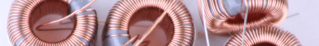
The second thing I remember was the zero-ripple Cuk converter. There was a transparency (pre-Powerpoint days!) where he rotated a picture of coupled cores and as the gap changed on the core, the ripple current flattened out to zero on the input and output. It was a great visual that really drove the point home.
And finally, he showed that the classic solution to the quadratic equation using the usual b2 – 4ac radical was numerically inaccurate, and he gave a much better solution.
I haven’t used his quadratic solution since then, nor have I designed with a coupled-inductor Cuk converter. But once I left his course I started measuring and understanding loop gains and found that they have never gone out of style for switching power supplies. Archaic though they seemed to me at the time, they are simply the best way to optimize the feedback of your power supply. Even if you are using a digital controller, an analog loop gain is simply the best way to verify that the feedback system is designed and working properly.
If you understand how to interpret loops properly, they are all you need for stability analysis. Text books talk about Nyquist plots, and characteristic equations, but in the real world we need to use the incredibly powerful tool for engineers that Mr. Bode gave to us. It is an amazing thing – with a couple of pen strokes on paper showing the loop gain and phase, we can determine the stability of systems of almost any order. What a potent engineering tool, no math needed, no calculus, only lab measurements! This was the great contribution of Bode.
The great contribution of Bode was that he enabled engineers to draw a couple of lines on a sheet of paper and declare whether a highly-complex, high-order, nonlinear system was stable or not! No match, no calculus needed. What more could we ask for?
The aerospace design world is probably the most rigorous in making complete sets of bode plots for input impedance, output impedance, audiosusceptibility, and loop gain. Outside of the aerospace world, it is less common to make this full set of measurements. Most experienced designers will make a loop gain measurement since they find that it is a very sensitive measure of just about everything in the power stage and the feedback path. If some component is the wrong value, or something is built wrong, the loop gain is very likely to show that there is a problem.
Critical Regions of a Voltage-Mode Loop Gain Measurement
When talking about loop gains, most articles refer to just the crossover frequency and the phase margin at that frequency. In reality, there is far more to a loop gain, and if you want to derive maximum benefit from making these measurements, it is important to understand where to look.
Figure 1 shows a typical loop gain for a voltage-mode power supply. The plot of Figure 1 starts at 10 Hz. This is always recommended, regardless of your power system switching frequency. It is very common to have substantial noise in the first decade of measurement (audio people are painfully aware of this, regarding hum) and you must be able to verify that you have high gain in the low frequency regions to reject line and other low-frequency noise. This area is shown shaded in blue in Figure 1. The AP300 frequency response analyzer [2,3] is capable of measuring gains in excess of 90 dB in the presence of high noise, and this is crucial for resolving high performance systems properly.
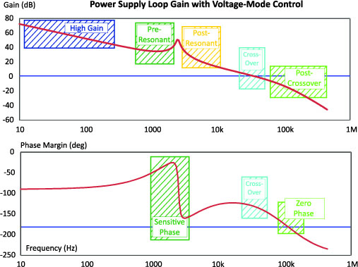
Figure 1: Voltage-Mode Loop Gain and Phase, Showing Key Measurement Regions.
There is a lot more to loop gain than just crossover frequency and phase margin. It is best to do a full swep from 10 Hz to twice the switching frequency to make sure you have captured everything in the system.
The green highlighted region in the loop gain of Figure 1 shows the region just before the resonant frequency of voltage-mode control. Because of the two compensation zeros in the feedback loop, and the high-Q double pole, there is a dip in the gain in this region. It is important that this gain is kept well above 20 dB to provide good transient performance.
Right after the resonance, the phase of the loop will drop very quickly and it will be very sensitive to changes in damping and loading. It is best to cross the loop over well beyond the filter resonance if you want to have a well-behaved system.
At the crossover frequency, shown in light blue region, we measure the phase margin of the system, and this gives an indication of the relative stability. It is recommended to have at least 50 degrees of phase margin under all conceivable operating conditions at the crossover frequency.
(Some people insist on not doing a loop gain measurement almost as a matter of principle. If you are relying on step-load transients to determine the phase margin, you are really only getting indirect information about the loop gain in the region of the crossover. This is not sufficient to optimize your system or to ensure it will always be stable. [1]. The same is true of output impedance measurements – they are not an adequate replacement for making a real loop-gain measurement.)
It is important to measure the loop gains well beyond the crossover frequency, as indicated in the light green region of Figure 1. You want to be sure that the gain in this region is monotonically decreasing. Even though the loop is below zero dB, it can still have an effect on the closed-loop output impedance of the system as will be shown below for a current-mode loop.
Critical Regions of a Current-Mode Loop Gain Measurement
Figure 2 shows a typical loop gain for a current-mode system. Again we start at 10 Hz to cover the low frequency noise region. Gains are much higher at low frequencies with current-mode control, and this provides outstanding closed-loop noise rejection.
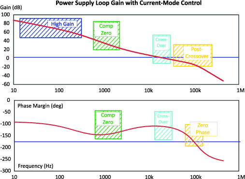
Figure 2: Current-Mode Loop Gain and Phase, Showing Key Measurement Regions.
The green region of the curve shows where the compensation zero of current-mode comes into play. Unlike voltage-mode control, there is no resonant frequency, and no need to match power stage poles with compensation zeros. We just put the compensation zero before the crossover frequency to make sure that we pull up the phase at crossover.
Notice the dip in the phase in this region. It is possible to avoid this dip by moving the compensation zero to a lower frequency, but this will result in lower gains at low frequency and less-than optimal performance.
As with voltage-mode control, we want to have a phase margin in excess of 50 degrees. The plot is continued well past crossover to make sure there is sufficient gain margin (what the gain is when the phase margin hits zero.) If you do not have a good gain margin, the closed-loop characteristics can show peaking, as shown in Figure 3.
Most designers are not aware that the loop gain still has an effect on performance even after it crosses over 0 dB. But as can be seen in the area circled in yellow, there is a peaking in the output impedance after the crossover frequency. This output impedance peaking has nothing to do with the phase margin of the power supply control loop which is more than adequate in this case.
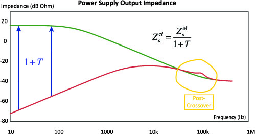
Figure 3: Open- and Closed-Loop Output Impedance
Summary
Loop gain measurements are potent tools for optimizing your system and making sure everything is working properly. It is important to look beyond just the crossover frequency and the phase margin of the loop gain, this is just a part of the story. This article has explained the importance of the low-frequency measurements and the importance of continuing the loop gain measurements well after the crossover frequency.
References
Readers are encouraged to view the videos listed below to learn more about making these measurements [5].
- Join our LinkedIn group titled “Power Supply Design Center”. Noncommercial site with over 7000 helpful members with lots of theoretical and practical experience.
- For power supply hands-on training, please sign up for our workshops.
- Step-Load Testing [Articles 29-30]