


Part I: Learn how to emulate the RidleyBox and AP310 Analyzers in LTspice®.
Authors: Dr. Ray Ridley, Art Nace and John Beecroft
Ridley Engineering, Inc. Camarillo, California USA
Introduction
Unpredictable and widely varying power stages and controllers demand measurements in the lab to confirm proper and reliable design information. The same techniques can be applied to simulation of your circuits. In this article, we describe a fast and high-performance frequency response analyzer circuit model for LTspice®. This model uses past foundational work by Mike Engelhardt [2] coupled with our advanced knowledge of the real-world functioning of hardware analyzers.
This gives access to the following:
1) Fast and clean simulation of the Bode plots,
2) Predictions for circuits that have no small-signal model available, and
3) Better results than small-signal models
Hardware Laboratory Instruments
There are more frequency response analyzers available on the market now than when I began in the power electronics business in 1981. Two of the best are the AP Instruments Model 310 analyzer from AP Instruments, and the new RidleyBox® from Ridley Engineering. These two products span the range of analyzers from a high-end product to a complete and affordable product solution.
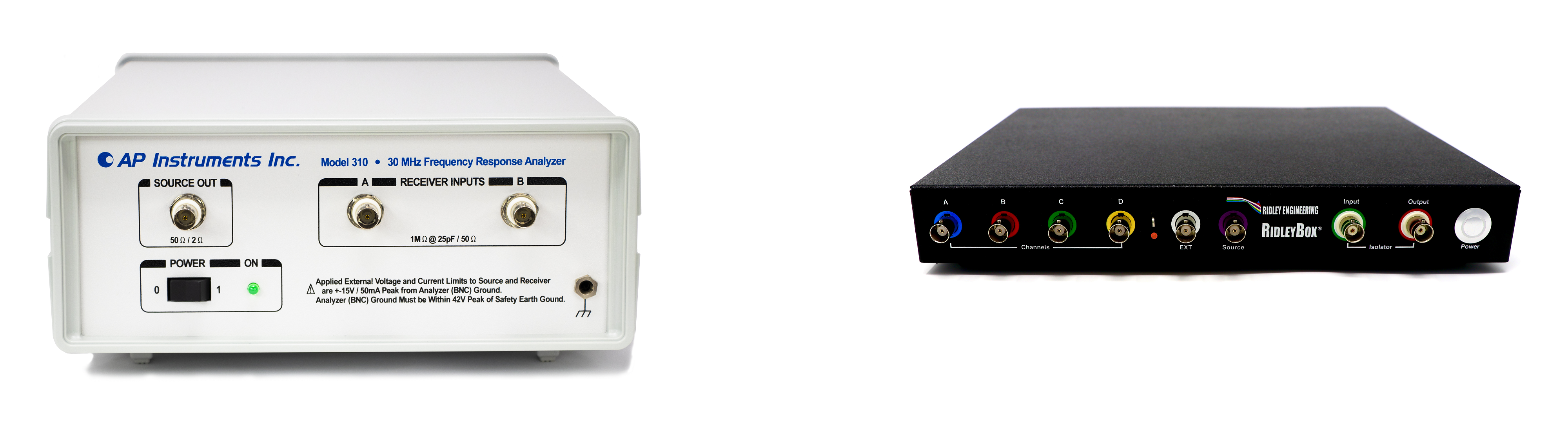
AP310 and RidleyBox Test Equipment
The features of the AP310 are crucial for obtaining reliable noise-free measurements. There is much to be learned from this analyzer that we will apply to achieve good results in the LTspice models within this article. We also implemented as many of these features and techniques as possible to the RidleyBox. In this article we will show how to emulate these analyzers in LTspice® models. You can learn more about other analyzers and measurement techniques in reference [1].
Emulating Frequency Response Analyzers in LTspice
The paper in reference [2] describes the fundamental techniques used for measuring transfer functions in LTspice®. For a test example, we set up a 100 kHz buck converter operating with voltage-mode control. The analyzer was first set up with the original suggestions in [2], not using any of our advanced features. The schematic of the test circuit is shown in Figure 1.
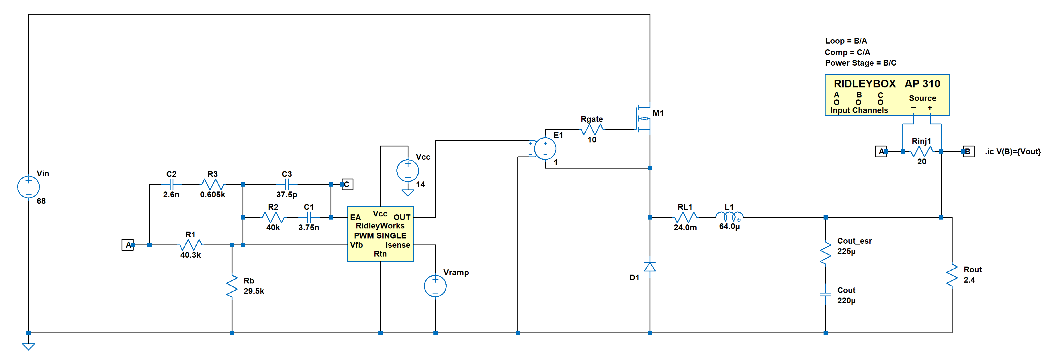
Figure 1: Buck converter test circuit with Frequency Response Analyzer subcircuit in LTspice®
Figure 2 shows the simulated output voltage of the converter as the analyzer sweeps from 100 Hz to 100 kHz. Each frequency is injected one at a time, and simulation waveforms are processed to extract the gain and phase response.
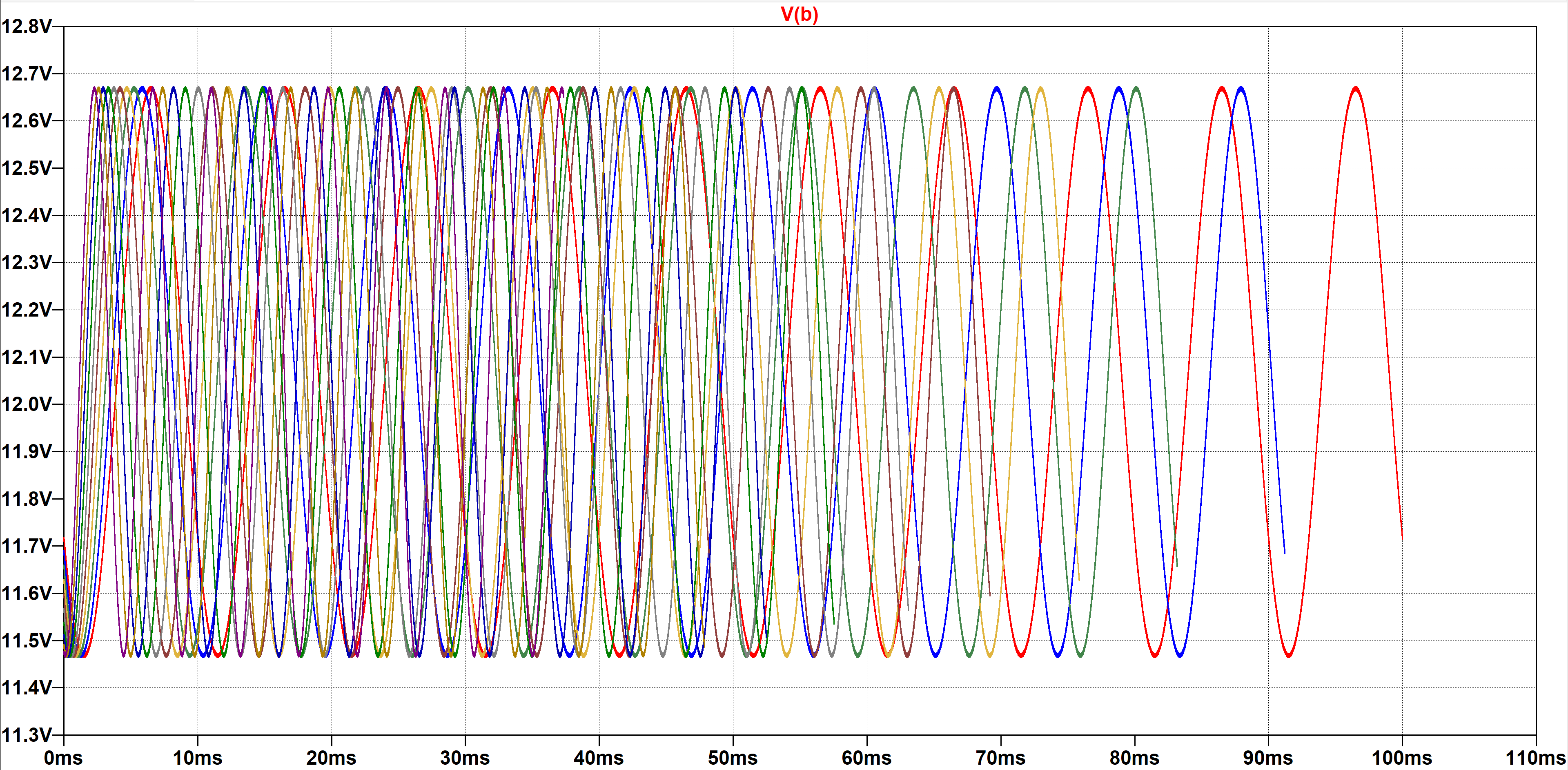
Figure 2: Typical simulation waveforms of original analyzer circuit and commands. Individual sinewaves are injected one at a time.
Figure 3 shows the loop gain plot that results from processing the simulated waveforms. This was done using the original settings proposed in [1] with a 10 mV signal and 10 cycles of each sinewave.
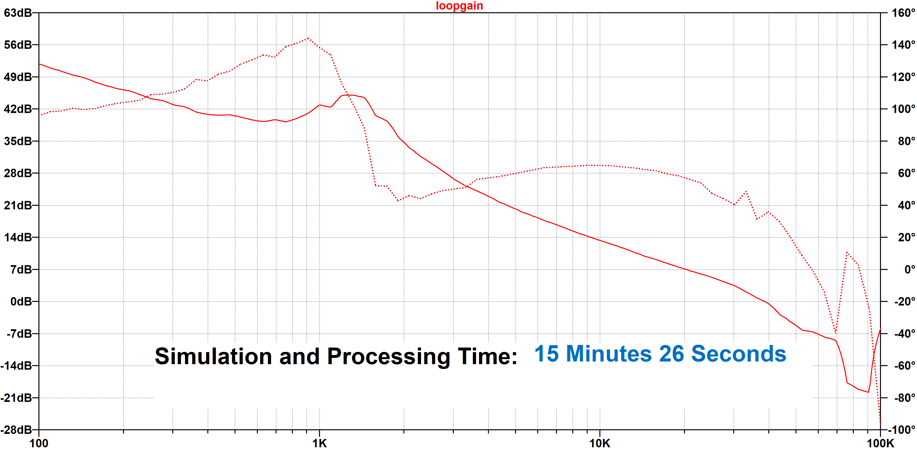
Figure 3: Loop gain using original paper settings (10 mV signal).
You can clearly see the problems in this plot. While the overall shape of the loop is present, there is a lot of noise at both low and high frequencies. This is not a curve that instills confidence in design credibility. The long processing time discourages further attempts at reducing the noise since this usually entails even longer simulation times.
In the original paper, one schematic suggests using 10 cycles of simulation at each frequency, and the other schematic suggests 25 cycles. The simulation of Figure 3 implemented 10 cycles, so we would anticipate a 37-minute simulation time with 25 cycles.
Anyone who has run a real frequency response analyzer in the lab on their hardware knows that the same kind of results are obtained if you do not have the instrument settings dialed correctly. We frequently see analyzers sitting unused on the shelf in companies and hear the comment that “no one remembers how to use it properly”.
The same is true for the simulation of the swept loop gain in LTspice®. You have to know how to control the emulated instrument properly. We have introduced 7 new control parameters to the analyzer setup to emulate the features of the AP Instruments analyzer and the RidleyBox. These new controls are:
1) Start Amplitude
2) Finish Amplitude
3) Start Break Frequency
4) Stop Break Frequency
5) Dwell Time
6) Bandwidth
7) High Frequency Noise Reduction
The profound effect of these combined control settings can be seen in Figure 4. The swept loop gain is now perfectly smooth and can be reliably used for design and for worst-case analysis of a finished design. This is now a serious tool for the power designer.
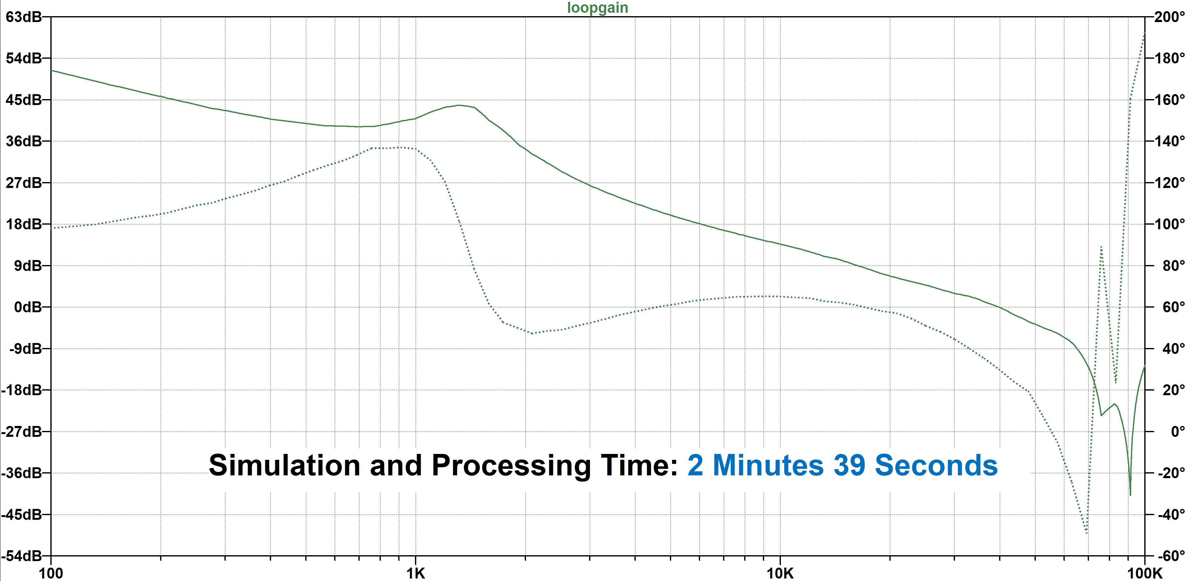
Figure 4: Swept loop gain using advanced analyzer settings and noise reduction.
In addition to the very smooth curves, there is a drastic reduction in the simulation and processing time. It is now under three minutes—six times better than the original analyzer settings. While smoothing out the curve is the main priority to make this a credible tool, we will see later that even faster sweeps are possible once this is done.
Advanced Analyzer Settings
In the world of analyzer hardware, AP Instruments introduced the first variable and programmable source in 1995. This was implemented at our request since we knew it was crucial to change the source size with frequency as you sweep a loop. That experience was learned after many years working in front of an HP4194A where you had to constantly adjust the source size while the loop was sweeping.
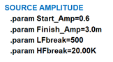
The same feature must be implemented in the software version of a good frequency response analyzer if you expect to see good results. Figure 5 shows how the source varies with frequency as you sweep from low to high values. In this example, the initial injection is 2 V, and the final value is 0.1 V. For the sweep in Figure 3, the initial set point was 0.6 V, and the final value is a very small 3 mV. The system measured does not have a lot of phase margin, and the injection must be kept small to avoid nonlinearities and a distorted curve.
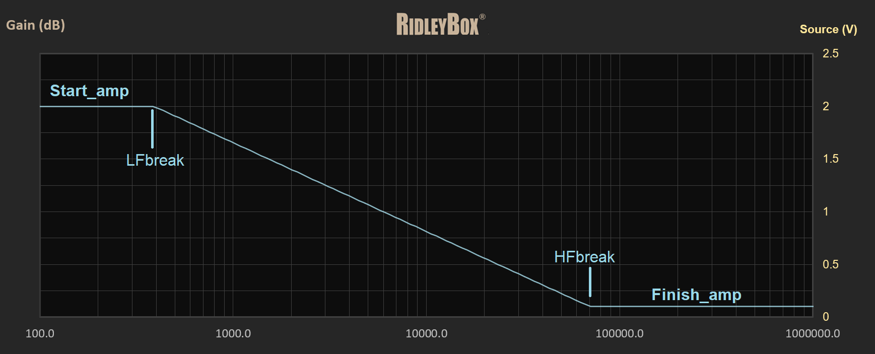
Figure 5: RidleyBox/AP310 LTspice® component variable source profile.
On the LTspice® schematic, the source is set with the following parameter commands, and the RidleyBox/AP310 component uses these values to adjust the source as the frequency is swept from low to high.
Start_Amp should not be larger than about 5% of the dc output voltage. A high value is needed here to be able to measure the very low input channel reliably.
Finish_Amp is a much smaller number—usually less than 10% of the start amplitude. For sensitive, low phase margin systems such as that in Figure 3, the value must be reduced until no distortion in the curve is observed. This is very much an empirical process, both in the lab with test hardware, or when using LTspice® to emulate the hardware.
LFBreak is the frequency at which the signal starts to reduce from its initial value. Typically, this is 1-10% of the anticipated crossover frequency.
HFBreak is the frequency at which the signal reaches its final value. This is usually just before the anticipated crossover frequency.
The measurement resolution is set with the following commands:
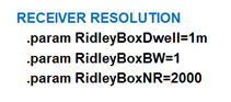
RidleyBoxDwell is the settling time after starting each new frequency. There must be enough time to allow the natural system transients to stabilize.
RidleyBoxBW determines the receiver bandwidth for the measurement channels. A low number indicates the fastest sweep. More difficult and noisy systems may require a higher number than 1 to improve the sweep smoothness.
RidleyBoxNR determines the frequency at which additional noise reduction is introduced. This technique is unique to the emulated analyzer and is not needed for hardware testing.
High-Speed Sweep Settings
When you are involved in design, you want sweeps to be as fast as possible for multiple iterations of a design. In this case, you can start at a frequency below the resonant frequency of the LC filter (to confirm its proper location) and use fewer data points. The curve is not quite as smooth, but you can see that it is more than sufficient for design with a sweep time under 30 seconds. This is truly amazing – LTspice® was never regarded as a practical platform for this kind of work in the past.
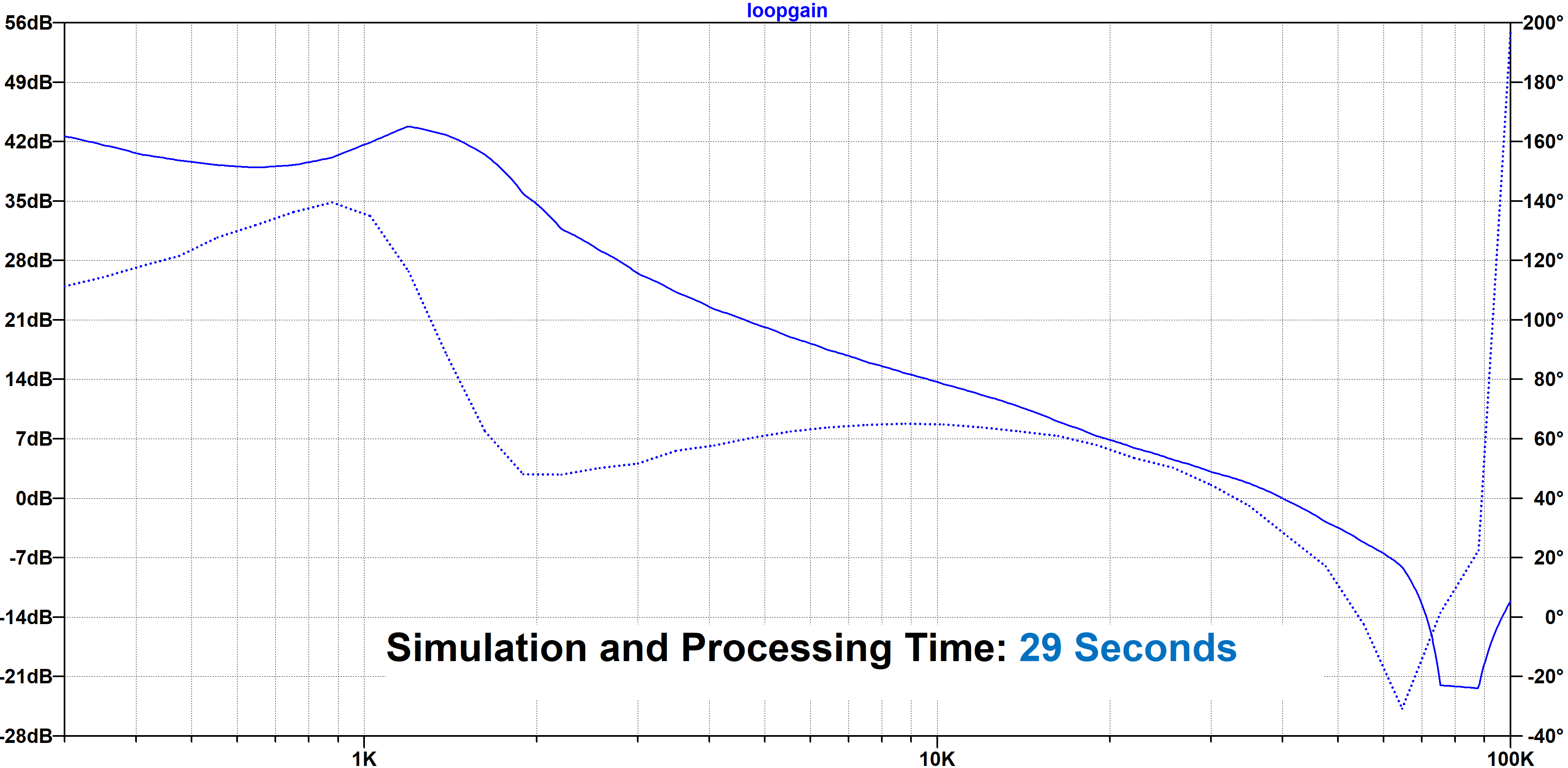
Figure 6: High-speed swept loop gain – start at 300 Hz, 15 points/decade
Summary
In this article we have shown that you can combine knowledge of frequency response analyzers with the features of LTspice® to obtain fast and dependable Bode plots for design and final system analysis. This is not a feature typically associated with LTspice®, and it opens up a new way to analyze systems without having small-signal models.
In the next article of this series, we will show how this approach will provide better results than small-signal models. We will also show how most small-signal models have fundamental limitations in their application to high-performance systems.
This should be a relief to many engineers. Deriving small-signal models is a very time-consuming process and accurate models simply do not exist for many systems.
References
[1] Frequency Response Measurement Two-Hour Masterclass. An extended training session with live measurement examples on switching power supplies. https://ridleyengineering.com/videos-e/315-frequency-response-measurement-masterclass.html
[2] Building a Frequency Response Analyzer in LTspice® by Mike Engelhardt
[3] Design and simulation using RidleyWorks®
[4] Hands-On Power Supply Design Workshops
[7] Join our LinkedIn group titled Power Supply Design Center. Noncommercial site with over 10,000 experienced and helpful industry experts.
[8] Join our Facebook group titled Power Supply Design Center. Advanced in-depth discussion group for all topics related to power supply design with over 5,000 industry experts .